Multiple Linear Regression applied to a Marketing Case Study

✅ Business Case

In this project, we are trying to predict sales revenues based on the budget invested into social media - Youtube, Facebook and some newspapers, using a multiple linear regression. The main focus of this project is to display how to validate the key assumptions of such a model. Get the full experience on my blog.

📉 Dataset

The dataset can be found on Kaggle. It describes the advertising experiment between Social Media Budget and Sales (in Thousands $ ) and hold 200 experiments.

📒 Repository

The repository is available on GitHub. It describes how to apply a Multiple Linear Regression Model using Scipy and how to perform regression diagnosis to validate the model.

🎯 Key take-away

Most firms that think they want advanced AI/ML really just need linear regression on cleaned-up data. [Robin Hanson]

There are four principal assumptions which support using a linear regression model for the purpose of inference or prediction:

1. Linearity:

We must have a linear relationship between our features and responses. This is required for our estimator and predictions to be unbiased. If you try to fit a linear model to data which is nonlinearly or nonadditive, your predictions are likely to be seriously in error, especially when you extrapolate beyond the range of the sample data. To confirm the linearity, we can for example, apply the Harvey-Collier multiplier test.

import statsmodels.stats.api as sms
sms.linear_harvey_collier(reg_multi)
>> Ttest_1sampResult(statistic=-1.565945529686271, pvalue=0.1192542929871369)

✅ A small p-value shows that there is a violation of linearity. Here the p-value is higher than the alpha risk (5%) meaning that the linearity condition is verified.

The next ones are concerning the residuals:

2. Normality:

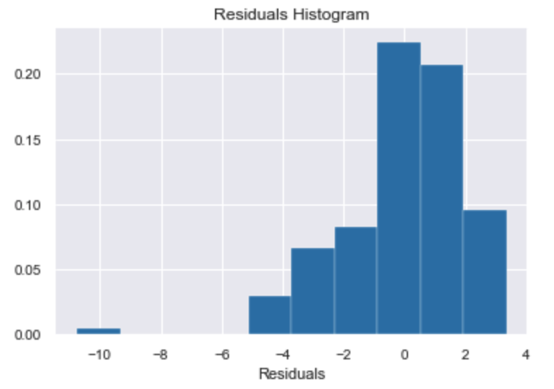
Residuals must be Normally distributed (i.e variance tend to 1 and mean tend to zero). This is necessary for a range of statistical tests, such as the t-test. We can relax this assumption in large samples due to the central limit theorem.

✅ If the residuals are normally distributed, we should see a bell-shaped histogram centered on 0 and with a variance of 1.

3. Homoscedasticity:

Means that the residuals have constant variance no matter the level of the dependent variable. We can use for example, the Breush-Pagan test. This test measures how errors increase across the explanatory variable.

import statsmodels.stats.api as sms
from statsmodels.compat import lzip
name = ['Lagrange multiplier statistic', 'p-value',
        'f-value', 'f p-value']
test = sms.het_breuschpagan(reg_multi.resid, reg_multi.model.exog)
lzip(name, test)
>> [('Lagrange multiplier statistic', 4.231064027368323),
 ('p-value', 0.12056912806125976),
 ('f-value', 2.131148563286781),
 ('f p-value', 0.12189895632865029)]

✅ If the test statistic has a p-value below the alpha risk (e.g. 0.05) then the null hypothesis of homoskedasticity is rejected and heteroskedasticity is assumed. In our case, we validate the assumption of homoscedasticity.

4. Independence:

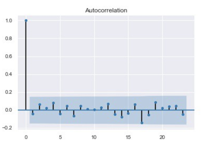
Residuals must be totally free of autocorrelation.

5. (…) And Multicollinearity

For multiple linear regression, you also need to check the absence of multicollinearity. Multicollinearity refers to when two predictors (or more) are providing the same information about the response variable. This can be a problem for the model as it generates:

• Redundancy → leading to unreliable coefficients of the predictors (especially for linear models)

• High variance of the estimator → tends to overfit meaning that the algorithm tends to model the random noise in the training data, rather than the intended output.

• An important predictor can become unimportant.

In other words, multicollinearity makes some variables statistically insignificant when they should be significant. We can check the existence of collinearity between two or more variables with the Variance Inflation Factor (VIF). It’s a measure of colinearity among predictor variables within a multiple regression.

We generally consider that a VIF of 5 or 10 and above (depends on the business problem) indicates a multicollinearity problem.

from statsmodels.stats.outliers_influence import variance_inflation_factor
from statsmodels.tools.tools import add_constant
# For each X, calculate VIF and save in dataframe
df.drop(['sales'],axis=1,inplace=True)
X = add_constant(df)
vif = pd.DataFrame()
vif["VIF Factor"] = [variance_inflation_factor(X.values, i) for i in range(X.shape[1])]
vif["features"] = X.columns
vif.round(1) #inspect results